library(plant)
library(parallel)

run <- function(seed_rain_in, p) {
  p$seed_rain <- seed_rain_in
  run_scm(p)$seed_rains
}

run_new_schedule <- function(seed_rain_in, p) {
  p$seed_rain <- seed_rain_in
  res <- build_schedule(p)
  attr(res, "seed_rain_out")
}

cobweb <- function(m, ...) {
  lines(rep(m[,1], each=2), c(t(m)), ...)
}

Try to establish what the equilibrium seed rain is.

Set model parameters

p0 <- scm_base_parameters("FF16")
p <- expand_parameters(trait_matrix(0.0825, "lma"), p0, FALSE)

Some output seed rains, given an input seed rain:

run(1.0, p)

## [1] 19.82443

run(10.0, p)

## [1] 17.63104

run(50.0, p)

## [1] 16.58796

When below the equilibrium, run returns a seed rain that is greater than the input, when above it, run returns a seed rain that is less than the input.

1: Approach to equilibrium:

p_eq <- equilibrium_seed_rain(p)

Equilibrium seed rain is right around where the last two values from run were producing

p_eq$seed_rain

## [1] 17.31512

From a distance, these both hone in nicely on the equilibrium, and rapidly, too.

approach <- attr(p_eq, "progress")
r <- range(approach)
plot(approach, type="n", las=1, xlim=r, ylim=r)
abline(0, 1, lty=2, col="grey")
cobweb(approach, pch=19, cex=.5, type="o")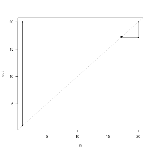

2: Near the equilibrium point:

Then, in the vicinity of the root we should look at what the curve actually looks like, without adaptive refinement.

dr <- 2 # range of input to vary (plus and minus this many seeds)
seed_rain_in <- seq(p_eq$seed_rain - dr,
                    p_eq$seed_rain + dr, length.out=31)
seed_rain_out <- unlist(mclapply(seed_rain_in, run, p_eq))

Here is input seeds vs. output seeds:

plot(seed_rain_in, seed_rain_out, xlab="Incoming seed rain",
     ylab="Outgoing seed rain", las=1, type="l", asp=5, col="red")
abline(0, 1, lty=2, col="grey")
cobweb(approach)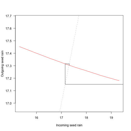

4. Global function shape

seed_rain_in_global <- seq(1, max(approach), length.out=51)

This takes quite a while to compute.

seed_rain_out_global <-
  unlist(mclapply(seed_rain_in_global, run_new_schedule, p))

This is pretty patchy, which is due to incompletely refining the cohort schedule, I believe. Tighten schedule_eps to make the curve smoother, at the cost of potentially a lot more effort.

plot(seed_rain_in_global, seed_rain_out_global,
     las=1, type="l",
     xlab="Incoming seed rain", ylab="Outgoing seed rain")
abline(0, 1, lty=2, col="grey")
cobweb(approach, lty=3)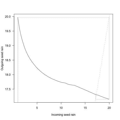

5. Multiple species at once:

lma <- c(0.0825, 0.15)
p2 <- expand_parameters(trait_matrix(lma, "lma"), p0, FALSE)

p2_eq <- equilibrium_seed_rain(p2)
approach <- attr(p2_eq, "progress")

From a distance, these both hone in nicely on the equilibrium, and rapidly, too.

r <- range(unlist(approach))
plot(approach[[1]], type="n", las=1, xlim=r, ylim=r, xlab="in", ylab="out")
abline(0, 1, lty=2, col="grey")
cols <- c("black", "red")
for (i in 1:2) {
  cobweb(approach[, i + c(0, 2)], pch=19, cex=.5, type="o", col=cols[[i]])
}
abline(v=p2_eq$seed_rain, col=1:2, lty=3)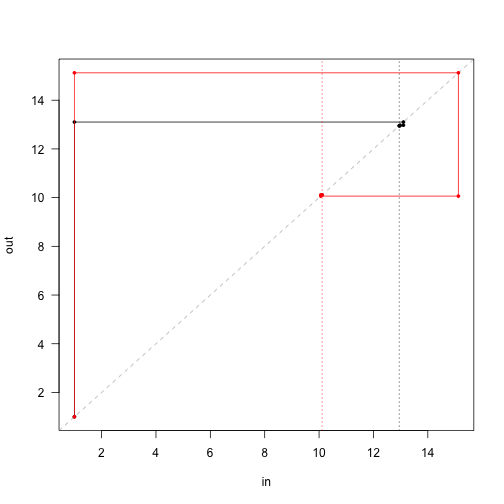

Note that the first guess position of the red species is higher than the black species, but in the end the output seed rain is lower. This is the difficulty in computing multi species equilibria - the different solutions affect each other. In general multi-dimensional root finding is difficult; even knowing that there are roots is not straightforward, much less proving that we’ve converged on the “correct” root (for example [0,0] is a root in this case but that root is not stable). plant uses some heuristics to try to ensure that the root returned is an attracting point but sequentially applying rounds of iteration and non-linear root finding algorithms, as well as rescaling seed rains to repel from known unstable roots.

To illustrate this a little further, though still in the fairly trivial 2d case, first identify the other two equilibria.

pp <- mclapply(lma, function(x)
  equilibrium_seed_rain(expand_parameters(trait_matrix(x, "lma"), p0, FALSE)))

Here’s the seed rains of each species when alone:

seed_rain1 <- sapply(pp, function(x) x$seed_rain)

So that means that we have four equilibria: 1: The trivial equilibrium:

eq00 <- c(0, 0)
run(eq00, p2_eq) - eq00

## [1] 0 0

2: Species 1 alone

eq10 <- c(seed_rain1[[1]], 0)
run_new_schedule(eq10, p2) - eq10

## [1] -0.009399603  0.000000000

3: Species 2 alone

eq01 <- c(0, seed_rain1[[2]])
run_new_schedule(eq01, p2) - eq01

## [1] 0.000000000 0.007976816

4: Species 1 and 2 together:

eq11 <- p2_eq$seed_rain
run(eq11, p2_eq) - eq11

## [1] 0.0011239196 0.0003123585

(note that the approximations here mean that these equilibria are not terribly well polished - there are a set of nested approximations that make this difficult. Possibly the biggest culprit is the cohort refinement step).

len <- 21
dx <- max(seed_rain1) / (len - 1)
n1 <- seq(0.001, by=dx, to=seed_rain1[[1]] + dx)
n2 <- seq(0.001, by=dx, to=seed_rain1[[2]] + dx)
nn_in <- as.matrix(expand.grid(n1, n2))
tmp <- mclapply(unname(split(nn_in, seq_len(nrow(nn_in)))),
                run_new_schedule, p2_eq)
nn_out <- do.call("rbind", tmp)

len <- log(rowSums(sqrt((nn_out - nn_in)^2)))
rlen <- len / max(len) * dx * 0.8

theta <- atan2(nn_out[, 2] - nn_in[, 2], nn_out[, 1] - nn_in[, 1])

x1 <- nn_in[, 1] + rlen * cos(theta)
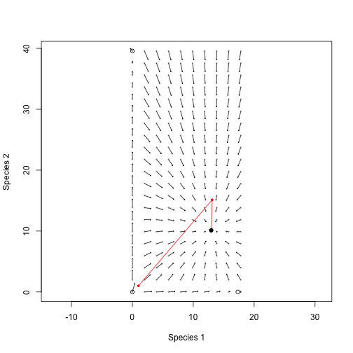
y1 <- nn_in[, 2] + rlen * sin(theta)

NOTE: I’m not sure why the point really close to the equilibrium here looks like it’s moving so quickly, and possibly in the wrong direction. Cohort instability perhaps?

plot(nn_in, xlab="Species 1", ylab="Species 2", pch=19, cex=.25,
     col="grey", asp=1)
arrows(nn_in[, 1], nn_in[, 2], x1, y1, length=0.02)
lines(rbind(approach[1, 1:2], approach[, 3:4]), type="o", col="red",
      pch=19, cex=.5)
points(p2_eq$seed_rain[[1]], p2_eq$seed_rain[[2]], pch=19)
points(rbind(eq00, eq10, eq01))